Multi-Layer Perceptron, MNIST 이해 및 개선해보기

MNIST 데이터와 함께 MLP 이해해보기

 

 

이번엔 미국의 인구조사국 직원들과 고등학생이 손으로 쓴 70,000개의 작은 숫자 이미지를 모은 MNIST 데이터 셋을 사용해서 기본적인 deep learning 방식인 MLP에 대해 공부해 보도록 합시다.

개발환경은 구글에서 제공하는 colab을 이용했습니다.

이번 실습환경에서는 pytorch와 numpy를 사용합니다.

다음과 같이 라이브러리를 다운받아 주세요.

# import libraries
import torch
import numpy as np

코드는 colab에서 실습해볼 수 있습니다.

 

 

데이터 내려받기

첫번째로 해야하는 일은 MNIST 데이터 셋을 내려받는 일입니다.

pytorch에서는 유명한 데이터 셋들을 내려받을 수 있도록 헬퍼함수를 제공합니다.
train data는 60,000개가 존재하며, test data는 10,000개가 존재합니다.

데이터를 20개씩 한 묶음으로 불러올 예정입니다. batch_size를 조정함으로써 한 묶음의 size를 변경할 수 있습니다.

각 데이터 세트에 대해서 DataLoader를 생성하도록 하겠습니다.

from torchvision import datasets
import torchvision.transforms as transforms

# number of subprocesses to use for data loading
# default가 0이며 0일경우 main process에서 작동합니다. 
num_workers = 0
# how many samples per batch to load
batch_size = 20

# convert data to torch.FloatTensor
# 이 함수를 사용하면 데이터들은 0과 1사이로 normalization 됩니다. 
transform = transforms.ToTensor()

# choose the training and test datasets
# 미리 지정된 url로 접근해서 train set과 test set을 불러옵니다. 
# transforms를 이용해 바로 텐서로 불러옵니다.
train_data = datasets.MNIST(root='data', train=True,
                                   download=True, transform=transform)
test_data = datasets.MNIST(root='data', train=False,
                                  download=True, transform=transform)

# prepare data loaders
train_loader = torch.utils.data.DataLoader(train_data, batch_size=batch_size,
    num_workers=num_workers)
test_loader = torch.utils.data.DataLoader(test_data, batch_size=batch_size, 
    num_workers=num_workers)

 

 

데이터 살펴보기

분류를 하기 전에 데이터의 특성을 살펴보는 것은 중요한 일입니다.
제대로 받아왔는지 확인해보고 data의 패턴이 어떤지 살펴봅시다.

import matplotlib.pyplot as plt
%matplotlib inline
    
# obtain one batch of training images
# iter는 객체의 __iter__ 메서드를 호출합니다. 
dataiter = iter(train_loader)
# next는 객체의 __next__ 메서드를 호출해줍니다. next를 두번 하면 두 번째 배치를 불러올 수 있습니다. 
images, labels = dataiter.next()  #next(dataiter)도 같은 동작을 제공합니다.  
images = images.numpy()

#image set을 살펴보면 20개의 image가 1*28*28의 형태로 담겨 있는 것을 확인할 수 있습니다. 
print(images.shape)


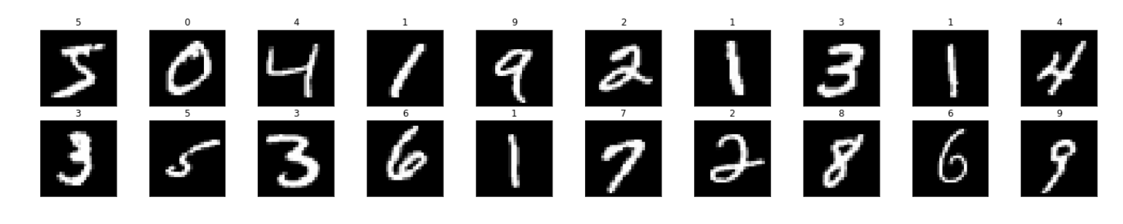
# plot the images in the batch, along with the corresponding labels
fig = plt.figure(figsize=(25, 4))
for idx in np.arange(20):
    ax = fig.add_subplot(2, 20/2, idx+1, xticks=[], yticks=[])
    ax.imshow(np.squeeze(images[idx]), cmap='gray')
    # 실제 label을 확인해보고 그림위에 나타내도록 하겠습니다. 
    # .item() gets the value contained in a Tensor
    ax.set_title(str(labels[idx].item()))

다음과 같이 지정한 배치 크기만큼 불러온 것을 확인 하실 수 있습니다.

 

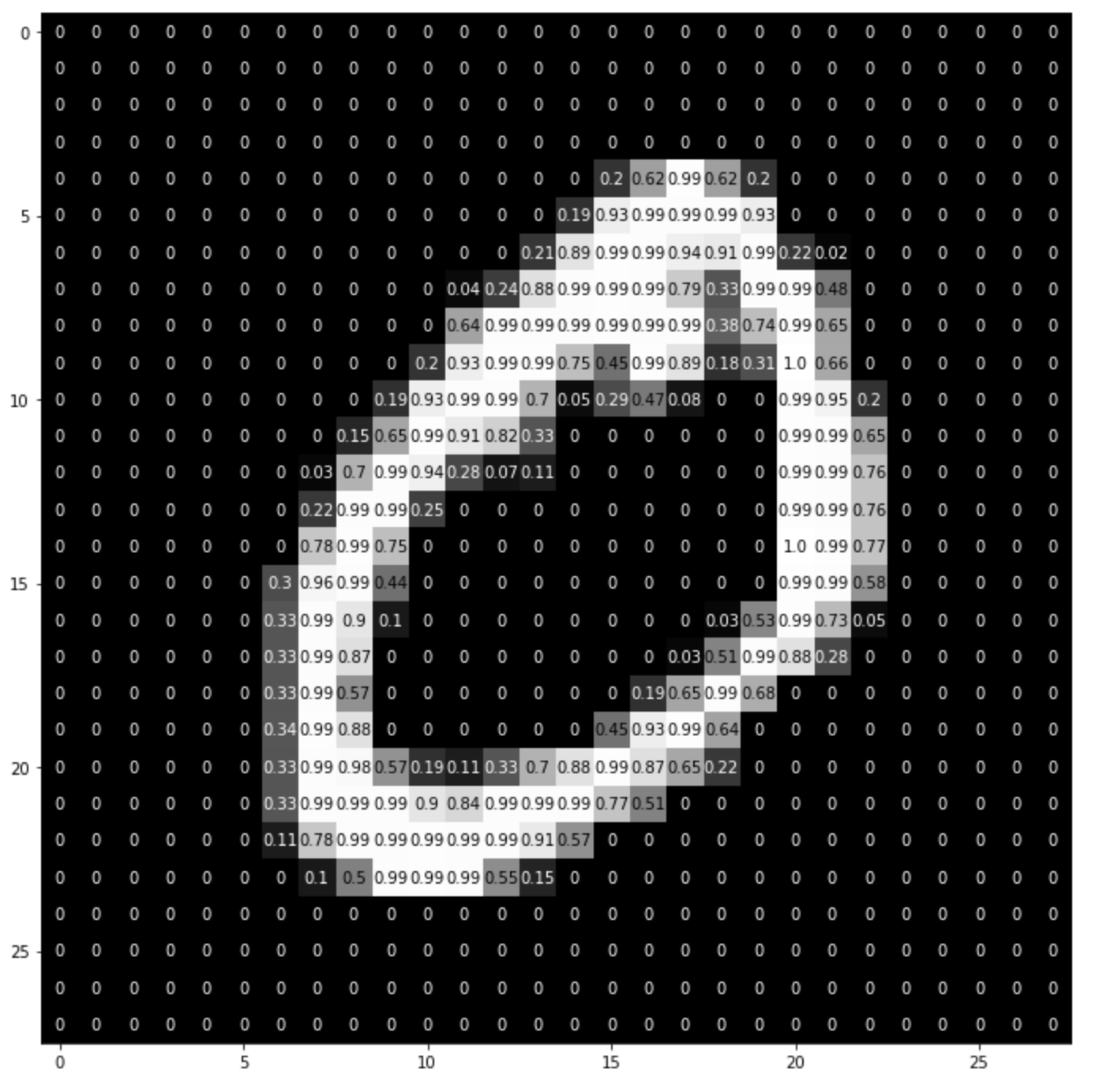
더 자세하게 이미지 살펴보기

# squeeze를 이용해서 크기가 1인 축을 없애 차원을 축소시킬 수 있습니다. 
img = np.squeeze(images[1])

fig = plt.figure(figsize = (12,12)) 
ax = fig.add_subplot(111)
ax.imshow(img, cmap='gray')
#이미지의 형태는 28*28 array
width, height = img.shape

thresh = img.max()/2.5
for x in range(width):
    for y in range(height):
        val = round(img[x][y],2) if img[x][y] !=0 else 0
        # 격자안 색이 thresh 이하일 경우 글자 색은 하얀색이 됩니다. 
        ax.annotate(str(val), xy=(y,x),
                    horizontalalignment='center',
                    verticalalignment='center',
                    color='white' if img[x][y]<thresh else 'black') 

위 코드를 실행하면 이미지의 구성이 다음과 같다는 것을 알 수 있습니다.

 

 

네트워크 아키텍처 구성하기

파이토치의 nn.Module을 사용하면 다음과 같이 간단하게 모델을 구축할 수 있습니다.
여기서 구성한 모델은 Multi-Layer Perceptron 구조입니다.
이미지의 픽셀들을 전부 받아와 모델의 input으로 넣습니다.
512개의 노드를 지닌 hidden layer를 통해 이미지의 고차원적인 특성을 학습하고
이후 10개의 카테고리로 나누기 위한 output layer를 지납니다.

이러한 과정은 forward 함수를 통해 설정해줄 수 있습니다.
본 예제에서는 결과 값이 0에 수렴하는 Vanishing Gradient 문제를 피하기 위해서
sigmoid 함수를 사용하지 않고 ReLU 함수를 활성화함수로 사용합니다.

sigmoid 함수를 hidden layer에 사용하게 되면
backward 과정에서 chain rule에 의해 점점 작은 값을 지니며 전파되게 됩니다.
그러므로 sigmoid 활성함수는 별다른 이유없이 hidden layer에서 사용되지 않습니다.

import torch.nn as nn
import torch.nn.functional as F

## Define the NN architecture
class Net(nn.Module):
    # 생성자에서 2개의 nn.Linear 모듈을 생성하고, 멤버변수로 지정합니다.
    def __init__(self):
        super(Net, self).__init__()
        self.fc1 = nn.Linear(28 * 28, 512)
        # linear layer (n_hidden -> 10)
        self.fc2 = nn.Linear(512, 10)

    # 순전파 함수는 입력데이터의 텐서를 받고 출력데이터의 텐서를 return해야 합니다. 
    # 텐서연산자와 생성자에서 정의한 모듈을 이용할 수 있습니다.
    def forward(self, x):
        # flatten image input
        x = x.view(-1, 28 * 28)
        # add hidden layer, with relu activation function
        x = F.relu(self.fc1(x))
        x = self.fc2(x)
        return x

# initialize the NN
model = Net()
print(model)

 

 

Loss Function과 Optimizer 정해주기

본 예제에서는 cross-entrophy를 분류문제에서 사용하도록 권장하고 있습니다. PyTorch에서의 cross entropy function은 결과에 softmax 함수를 적용시킨 후 log loss를 계산합니다. 유의해야할 점은 소프트맥스 분류기는 한번에 하나의 클래스만 예측한다는 것입니다. 하나의 사진에서 여러개의 물체를 동시에 인식하는 모델로는 사용할 수 없습니다.

cross-entrophy는 정보이론에서 유래했습니다. $2^n$ 만큼의 정보는 n-bit를 사용해 인코딩할 수 있습니다.
cross-entrophy는 타깃에 대해 낮은 확률을 예측하는 모델에 대해 비용을 높이는 성질을 지니고 있습니다. 자주 일어나지 않는 일이어야 하므로 그만큼 엔트로피를 높게 책정하는 것 입니다.
이러한 성질은 추정된 클래스의 확률이 타깃 클래스와 얼마나 부합하는지 측정하는 용도로 사용되기에 적합합니다.

## Specify loss and optimization functions

# specify loss function
criterion = nn.CrossEntropyLoss()

# specify optimizer
optimizer = torch.optim.SGD(model.parameters(), lr=0.1)

optimizer는 확률적 경사 하강법(Stochastic Gradient Descent)을 사용합니다.
이 방법은 전체 데이터의 loss를 구하는 것이 아닌 일부데이터를 가져와 loss를 계산하는 것으로 일부데이터로 연산을 진행하는 만큼 더 빠른 학습을 진행할 수 있습니다.
또한 결국 모든 데이터를 사용하기 때문에 Batch Gradient Descent의 결과로 수렴합니다.
모든 데이터에 대한 loss를 적용시키면 local minmima에 빠질 가능성이 있습니다. SGD를 쓰면 이러한 문제를 어느정도 회피할 수 있습니다.

 

 

네트워크 학습

네트워크는 다음과 같은 과정으로 학습됩니다.

1. 모든 변수에 대해 gradients를 초기화 시켜줍니다.
2. data를 모델에 전달하면서 전방향(forward) 연산을 진행합니다.
3. loss를 계산합니다. 이후 loss 정도에 따라 gradient를 조정합니다.
   이는 backward로 전파되며 진행됩니다.
4. optimizer를 통해 파라미터들을 업데이트 합니다.
5. 평균 training loss율을 보여줍니다.

# number of epochs to train the model
n_epochs = 10  # suggest training between 10-50 epochs

model.train() # prep model for training

# 한 번의 epoch를 진행한다는 것은 전체 데이터를 모두 둘러본다는 뜻입니다. 
for epoch in range(n_epochs):
    # monitor training loss
    train_loss = 0.0
    
    ###################
    # train the model #
    ###################
    for data, target in train_loader:
        # 1. clear the gradients of all optimized variables
        optimizer.zero_grad()
        # 2. forward pass: compute predicted outputs by passing inputs to the model
        output = model(data)
        # 3. calculate the loss
        loss = criterion(output, target)
        # backward pass: compute gradient of the loss with respect to model parameters
        loss.backward()
        # 4. perform a single optimization step (parameter update)
        optimizer.step()
        # 5. update running training loss
        train_loss += loss.item()*data.size(0)
        
    # print training statistics 
    # calculate average loss over an epoch
    train_loss = train_loss/len(train_loader.dataset)

    print('Epoch: {} \tTraining Loss: {:.6f}'.format(
        epoch+1, 
        train_loss
        ))

 

 

모델 테스트하기

이제 학습시킨 모델을 이용해 test를 해보겠습니다.
test set은 모델이 처음 보는 data set이어야 합니다.
전체 loss와 accuracy를 측정할 수 있습니다.

# initialize lists to monitor test loss and accuracy
test_loss = 0.0
class_correct = list(0. for i in range(10))
class_total = list(0. for i in range(10))

model.eval() # prep model for *evaluation*

for data, target in test_loader:
    # forward pass: compute predicted outputs by passing inputs to the model
    output = model(data)
    # calculate the loss
    loss = criterion(output, target)
    # update test loss 
    test_loss += loss.item()*data.size(0)
    # convert output probabilities to predicted class
    _, pred = torch.max(output, 1)
    # compare predictions to true label
    correct = np.squeeze(pred.eq(target.data.view_as(pred)))
    # calculate test accuracy for each object class
    for i in range(batch_size):
        label = target.data[i]
        class_correct[label] += correct[i].item()
        class_total[label] += 1

# calculate and print avg test loss
test_loss = test_loss/len(test_loader.dataset)
print('Test Loss: {:.6f}\n'.format(test_loss))

for i in range(10):
    if class_total[i] > 0:
        print('Test Accuracy of %5s: %2d%% (%2d/%2d)' % (
            str(i), 100 * class_correct[i] / class_total[i],
            np.sum(class_correct[i]), np.sum(class_total[i])))
    else:
        print('Test Accuracy of %5s: N/A (no training examples)' % (classes[i]))

print('\nTest Accuracy (Overall): %2d%% (%2d/%2d)' % (
    100. * np.sum(class_correct) / np.sum(class_total),
    np.sum(class_correct), np.sum(class_total)))

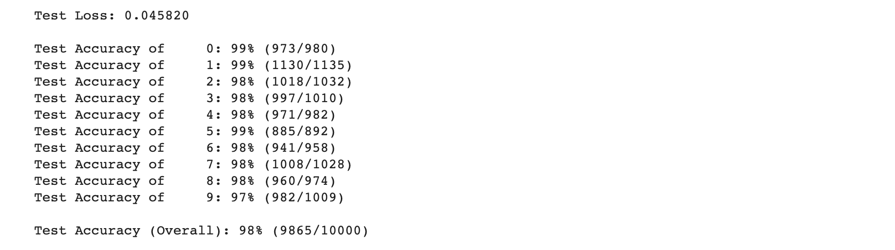
결과는 다음과 같습니다.

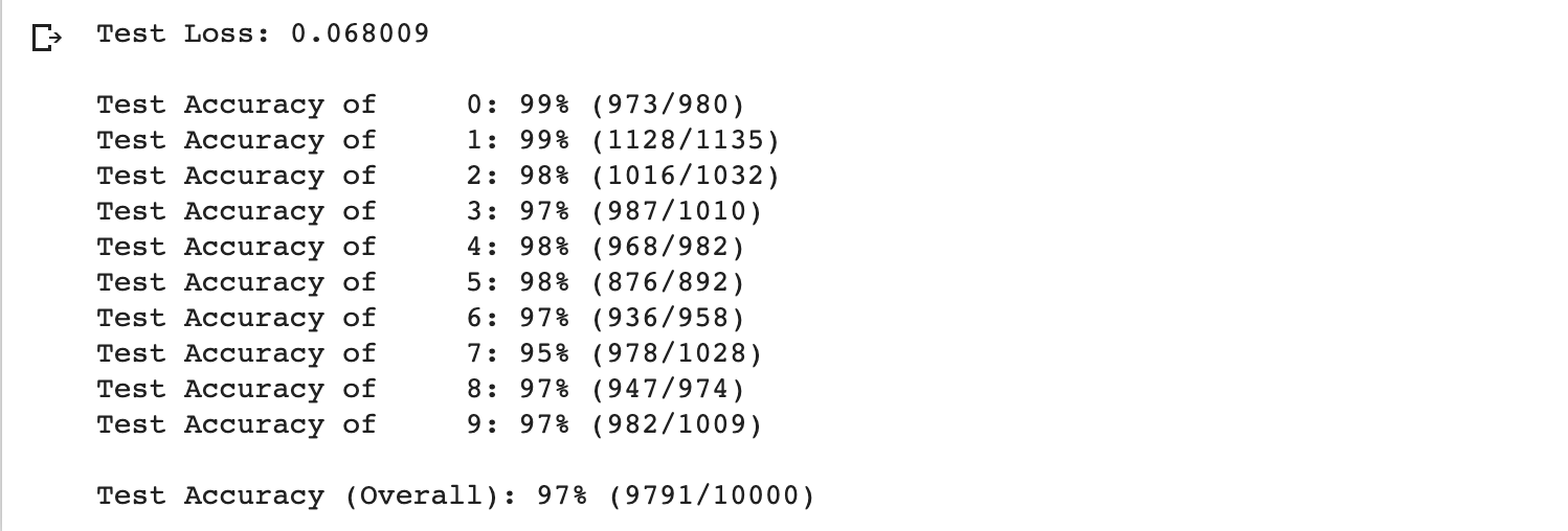
저희가 지금까지 학습한 모델은 97%의 정확도를 보여줍니다.

 

 

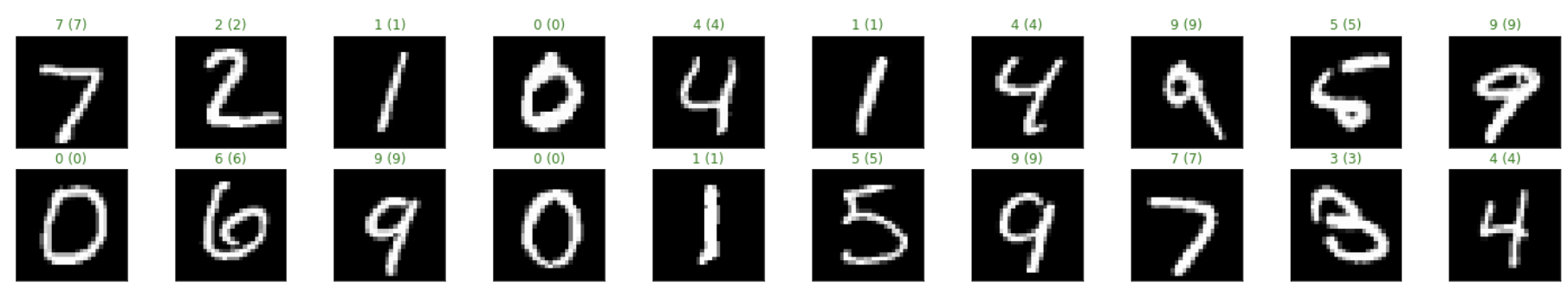
test 결과 시각화

다음과 같이 테스트의 결과를 시각화 할 수 있습니다.
시각화를 통해 어떤 유형의 데이터를 모델이 잘 학습하는지 알아볼 수 있습니다.

# obtain one batch of test images
dataiter = iter(test_loader)
images, labels = dataiter.next()

# get sample outputs
output = model(images)
# convert output probabilities to predicted class
_, preds = torch.max(output, 1)
# prep images for display
images = images.numpy()

# plot the images in the batch, along with predicted and true labels
fig = plt.figure(figsize=(25, 4))
for idx in np.arange(20):
    ax = fig.add_subplot(2, 20/2, idx+1, xticks=[], yticks=[])
    ax.imshow(np.squeeze(images[idx]), cmap='gray')
    ax.set_title("{} ({})".format(str(preds[idx].item()), str(labels[idx].item())),
                 color=("green" if preds[idx]==labels[idx] else "red"))

결과는 다음과 같습니다.

 

 

모델의 성능 높여보기

지금까지 MNIST 데이터와 함께 기본적인 MLP 모델에 대해 이해해보는 시간을 가졌습니다.

딥러닝 모델은 일반적인 문제를 해결하기 위해 과적합을 해결해야 합니다. 복잡한 모델일 수록 데이터의 특성에 민감해지기 때문에 이를 완화시켜줄 수 있는 방법을 찾아야 합니다.

기본적으로 딥러닝 모델은 학습데이터가 많으면 많을 수록 일반적인 문제를 잘 해결하게 됩니다.
규제화 혹은 학습의 learning rate를 조절하는 optimizer 역시 test set에 대한 모델의 성능에 영향을 미칩니다.

학습 데이터를 확장시켜보기

데이터를 더 늘리는 방식으로 data augmentation이라는 방법이 있습니다.
이는 데이터에 조금씩 변형을 가해서 가지고 있는 데이터로 새로운 데이터를 생성하는 방법을 말합니다.

pytorch에서는 torchvision.transforms 모듈에서 이미지의 형태를 지니고 있는 텐서를 쉽게 변환시켜주는 툴을 내장하고 있습니다.
지금부터 transforms를 이용해서 이미지를 좀 더 확장시켜보겠습니다.

RandAffine = transforms.RandomAffine(degrees=45, translate=(0.1, 0.1), scale=(0.8, 1.2))

rotate = transforms.RandomRotation(degrees=25)
shift = RandAffine
composed = transforms.Compose([rotate,
                               shift,
                               transforms.ToTensor()])

# number of subprocesses to use for data loading
num_workers = 0
# how many samples per batch to load
batch_size = 20

# convert data to torch.FloatTensor

# choose the training and test datasets
train_data2 = datasets.MNIST(root='data', train=True,
                                   download=True, transform=composed)

#원래 존재하는 train set과 붙여줍니다. 
train_data = torch.utils.data.ConcatDataset([train_data2, train_data])

# prepare data loaders
train_loader = torch.utils.data.DataLoader(train_data, batch_size=batch_size, num_workers=num_workers)

변형시키기 전의 데이터의 모습이 다음과 같다면,

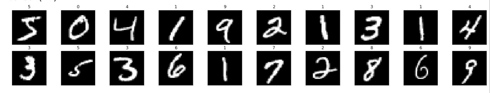
변형 후의 이미지들은 다음과 같습니다.

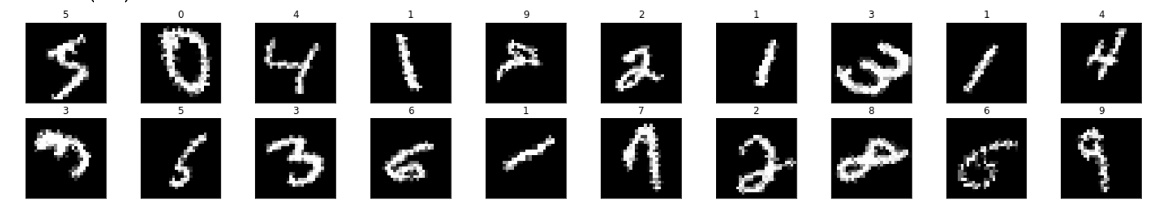
이렇게 확장시킨 data set을 사용해서 같은 모델로 학습을 진행해 줍니다.
dataset이 더 많아졌기 때문에 학습의 시간은 더 오래걸릴 것 입니다.

# number of epochs to train the model
n_epochs = 10  # suggest training between 10-50 epochs

model.train() # prep model for training

for epoch in range(n_epochs):
    # monitor training loss
    train_loss = 0.0
    
    ###################
    # train the model #
    ###################
    for data, target in train_loader:
        # clear the gradients of all optimized variables
        optimizer.zero_grad()
        # forward pass: compute predicted outputs by passing inputs to the model
        output = model(data)
        # calculate the loss
        loss = criterion(output, target)
        # backward pass: compute gradient of the loss with respect to model parameters
        loss.backward()
        # perform a single optimization step (parameter update)
        optimizer.step()
        # update running training loss
        train_loss += loss.item()*data.size(0)
        
    # print training statistics 
    # calculate average loss over an epoch
    train_loss = train_loss/len(train_loader.dataset)

    print('Epoch: {} \tTraining Loss: {:.6f}'.format(
        epoch+1, 
        train_loss
        ))

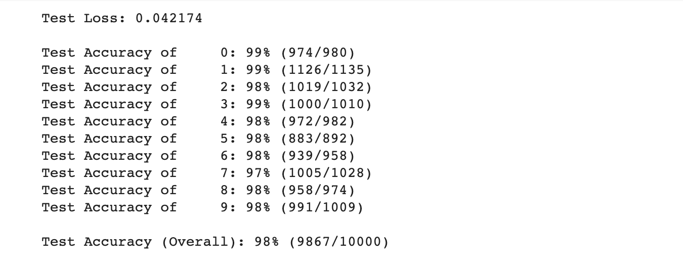
학습의 loss 결과는 다음과 같습니다.

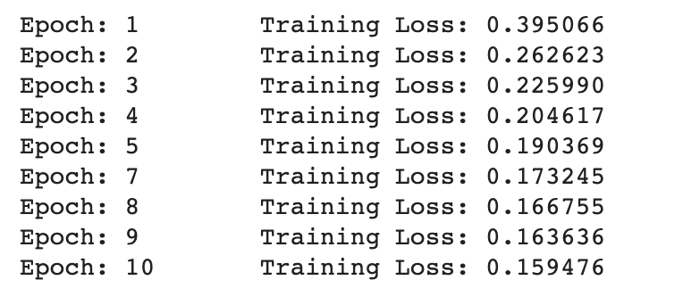
똑같이 검증을 진행해보면 데이터를 추가하지 않았을 때보다 1%의 성능이 더 향상된 것을 볼 수 있습니다.

 

모델을 변경해보기 + GPU 사용해보기

간단하게 모델을 변경시키는 방법은 다음과 같습니다.

1. 레이어의 갯수를 변경시켜본다. (과대적합이 될 수 있습니다.)
2. dropout을 진행한다. (과소적합이 될 수 있습니다.)
3. optimizer를 변경한다.

위와 같은 변경방법은 프레임워크가 이미 제공하고 있어 간단하게 적용할 수 있습니다.
적용한 모습은 다음과 같습니다.

추가적으로 torch에서 gpu를 활용해보는 코드를 추가해봅시다.

#optimizer에 따른 적정 learning rate는 모두 다르므로 주의해주세요.
optimizer_adam = torch.optim.Adam(model2.parameters(), lr=1e-3)

import torch.nn as nn
import torch.nn.functional as F

class Net2(nn.Module):

    def __init__(self):
        super(Net2, self).__init__()
        self.fc1 = nn.Linear(28 * 28, 512)
        # linear layer (n_hidden -> 10)
        self.fc2 = nn.Linear(512, 120)
        self.fc3 = nn.Linear(120, 84)
        self.fc4 = nn.Linear(84, 10)

    def forward(self, x):
        # flatten image input
        x = x.view(-1, 28 * 28)
        # add hidden layer, with relu activation function
        x = F.relu(self.fc1(x))
        # dropout을 통해 임의의 파라미터를 선택해 집중적으로 학습시킬 수 있습니다.
        x = F.dropout(x, p=0.3)
        x = F.relu(self.fc2(x))
        x = F.relu(self.fc3(x))
        x = self.fc4(x)
        return x

# initialize the NN
model2 = Net2()
# 모델을 gpu로 넣어줍니다.
if torch.cuda.is_available():
    model2.cuda()
print(model2)

n_epochs = 10

model2.train() # prep model2 for training

for epoch in range(n_epochs):
    # monitor training loss
    train_loss = 0.0
    
    ###################
    # train the model2 #
    ###################
    for data, target in train_loader:
        # cuda를 사용하기 위해 데이터를 gpu로 넣어줍니다. 
        if torch.cuda.is_available():
            data = data.cuda()
            target = target.cuda()
        # clear the gradients of all optimized variables
        optimizer_adam.zero_grad()
        # forward pass: compute predicted outputs by passing inputs to the model
        output = model2(data)
        # calculate the loss
        loss = criterion(output, target)
        # backward pass: compute gradient of the loss with respect to model parameters
        loss.backward()
        # perform a single optimization step (parameter update)
        optimizer_adam.step()
        # update running training loss
        train_loss += loss.item()*data.size(0)
        
    # print training statistics 
    # calculate average loss over an epoch
    train_loss = train_loss/len(train_loader.dataset)

    print('Epoch: {} \tTraining Loss: {:.6f}'.format(
        epoch+1, 
        train_loss
        ))

위와 같이 학습을 진행하고 얻은 결과는 다음과 같습니다.

일반적인 모델로는 98%까지의 성능을 낼 수 있었습니다.
data를 더 잘 조정한다면 99% 성능까지도 보일 수 있을 것 같습니다.

일반적으로 이미지를 분류하는 모델에서 가장 좋은 성능을 보인 모델은 CNN모델입니다.
이 모델을 사용하면 99%의 정확도를 지닌 모델을 만들 수 있습니다.

관련 포스팅은 추후에 진행학도록 하겠습니다.

 

 

번외 : tensorflow2 케라스로 구현한 동일 모델

텐서플로2에서 제공하는 케라스 모듈을 이용해서 간단하게 같은 모델을 만들 수 있습니다.
과정은 위에서 본 것들을 동일하게 적용시켰습니다.

colab을 통해 실습을 진행해 보실 수 있습니다.

!pip install -q tensorflow-gpu==2.0.0-rc1
import tensorflow as tf

from tensorflow.python.client import device_lib 

device_lib.list_local_devices()
tf.test.is_gpu_available()

%matplotlib inline
import matplotlib.pyplot as plt
import matplotlib.cm as cm

import numpy as np

mnist = tf.keras.datasets.mnist

(x_train, y_train), (x_test, y_test) = mnist.load_data()
#normalize dataset
x_train, x_test = x_train / 255.0, x_test / 255.0

# display image
def display(img):
    
    plt.axis('off')
    plt.imshow(img, cmap=cm.binary)

# output image     
display(x_train[0])

from imgaug import augmenters
# Adding image rotation, shift, zoom
augs_one = []
for i in x_train:
    rotate = augmenters.Affine(translate_percent={"x": (-0.1, 0.1), "y": (-0.1, 0.1)}, rotate=(-15, 15),
                               scale={"x": (0.9, 1.1), "y": (0.9, 1.1)})
    aug_image = rotate.augment_image(i)
    augs_one.append(aug_image)

# Review Augmented Images
width = 6
height = 6
fig = plt.figure(figsize = (width, height))
columns = 4
rows = 5
for i in range(1, columns * rows + 1):
    fig.add_subplot(rows, columns, i)
    plt.imshow(augs_one[np.random.randint(low = 0, high = 784)], cmap='Greys_r')
plt.show()

augs_one = np.asarray(augs_one)
x_train_append = np.append(x_train, augs_one, axis=0)
y_train_append = np.append(y_train, y_train, axis=0)

model = tf.keras.models.Sequential([
  tf.keras.layers.Flatten(input_shape=(28, 28)),
  tf.keras.layers.Dense(128, activation='relu'),
  tf.keras.layers.Dropout(0.2),
  tf.keras.layers.Dense(10, activation='softmax')
])

model.compile(optimizer='Adam',
              loss='sparse_categorical_crossentropy',
              metrics=['accuracy'])

tf.keras.utils.plot_model(model, show_shapes=True)

model.fit(x_train_append, y_train_append, batch_size=20, epochs=10)

model.evaluate(x_test,  y_test, verbose=1)